This submission is courtesy of Dr. Heather Matthees, Research Soil Scientist, USDA-ARS, Morris, MN. It was originally published in the AGVISE Newsletter Fall 2017.
Salt-affected soils are a major problem for agricultural producers, resulting in $12 billion annual losses in crop production across the world. In the northern Great Plains and Canadian Prairies, soil salinity has always existed in some soils of the region, but the problem has become more widespread and severe since a hydrological wet period began in the 1990s.
Salinity is the overall abundance of soluble salts, which compete with plant water uptake and reduce crop productivity. The soluble salts pull soil water toward themselves in the soil solution, which leaves less soil water available for plant uptake. This causes an apparent drought stress, reducing crop productivity and sometimes may kill the plant. Soluble salts are naturally occurring and a product of regional geology in the northern Great Plains and Canadian Prairies. Since the 1990s, the hydrological wet period has raised the groundwater level and allowed saline groundwater to rise toward the soil surface, causing soil salinization. Saline soils are often called “salty,” “sour”, or “white alkali.”
The severity of soil salinity will control which plant species are suitable for crop or forage production. Some crop species like dry bean and soybean are very sensitive to salinity, whereas other crop species like barley and sunflower have good tolerance to salinity. For soils with very high salinity, the only practical forage option may be salt-tolerant perennial grasses. To assess soil salinity, there are two soil analysis methods: saturated paste extraction and routine 1:1 soil water methods.
Saturated Paste Extraction Method
The gold standard in soil salinity research is the saturated paste extraction method. The method requires a trained laboratory technician to mix soil and water into a paste, just reaching the saturation point, which is about the consistency of pudding. The saturated paste rests overnight to dissolve the soluble salts. It is then is placed under vacuum to draw the saturated paste extract. Soil salinity is then determined by measuring the electrical conductivity (EC) of the saturated paste extract.
The saturated paste extraction method is fairly straightforward, but it requires a trained technician, specialized equipment, and over 24 hours to complete the procedure. The procedure is labor intensive and difficult to automate, so it is considered a special analysis service in commercial soil testing. Therefore, it is more expensive than routine soil testing methods. Among soil salinity determination methods, it is considered the most accurate because the soil:water ratio at saturation controls for differences in soil texture and water holding capacity.
Routine 1:1 Soil:Water Method
The routine method for soil salinity assessment is the 1:1 soil:water method, which mixes standard mass of soil (10 g) and volume of water (10 mL) in a soil-water slurry. Soil salinity is then determined by measuring the electrical conductivity (EC) of the soil-water slurry. It is most commonly abbreviated EC1:1.
The method is fast and inexpensive (only 5-10% of saturated paste extraction cost). The low cost per soil sample allows a person to collect more soil samples from various soil depths and multiple locations within a field (e.g. zone soil sampling), which can create a more comprehensive and detailed soil salinity map to evaluate soil salinity presence, severity, and variability. Since soil salinity is so intimately related to soil water movement across the landscape, the soil salinity map also provides information about soil water accumulation and leaching, soil nutrient movement (e.g. chloride, nitrate-nitrogen, sulfate-sulfur), and crop productivity potential.
A general caveat about the 1:1 soil:water method is that the reported values will be lower than the saturated paste extraction method. Fortunately, the two methods are highly correlated. AGVISE Laboratories worked with soil science researchers at North Dakota State University and South Dakota State University to validate the correlation between the two methods using over 2,300 soil samples from the northern Great Plains. You can convert the two methods by multiplying the 1:1 soil:water result by 2.26 to estimate the saturated paste extraction result (Figure 1).
The simple method conversion enables you to quickly and cheaply monitor soil salinity using the 1:1 soil:water method and still utilize the historical soil salinity interpretation criteria based on the saturated paste extraction method.
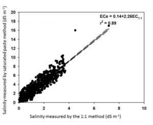
Figure 1. Soil salinity method conversion between saturated paste extraction and 1:1 soil:water methods.
References
Matthees, H. L., He, Y., Owen, R. K., Hopkins, D., Deutsch, B., Lee, J., Clay, D. E., Reese, C., Malo, D. D., & DeSutter, T. M. 2017. Predicting soil electrical conductivity of the saturation extract from a 1:1 soil to water ratio. Communications in Soil Science and Plant Analysis, 48(18), 2148–2154.
Starter Fertilizer Display: How low can YOU go?
in Canola, Corn, Phosphorus, Soybean, Starter Fertilizer, Sugar Beet, Wheat/by John LeeWhen profits are squeezed, more farmers are asking about optimal starter fertilizer rates and how low starter fertilizer rates can be. These questions are the result of wanting to keep fertilizer costs down, to plant as many acres per day as possible, and to take advantage of more efficient, lower rates of banded phosphorus fertilizer compared to higher rates of broadcast phosphorus fertilizer.
The displays show the normal seed spacing for several crops with different dry or liquid fertilizer rates alongside the seed. These displays help visualize the distance between the seed and fertilizer at several rates. University research shows that to achieve the full starter effect, a fertilizer granule or droplet must be within 1.5-2.0 inches of each seed. If the fertilizer granule or droplet is more than 1.5-2.0 inches away from the seed, the starter effect is lost. Some people wonder about these displays, but you can prove it to yourself pretty easily. Just run the planter partially down on a hard surface at normal planting speed. You will see what you imagine as a constant stream of liquid fertilizer, ends up being individual droplets at normal speed, especially with narrow row spacings and lower fertilizer rates.
These displays help illustrate the minimum starter fertilizer rate to maintain fertilizer placement within 1.5-2.0 inches of each seed for the full starter effect. In addition to an adequate starter fertilizer rate, additional phosphorus and potassium should be applied to prevent nutrient mining, causing soil test levels to decline in years when minimum fertilizer rates are applied.
Adjusting low soil pH with sugar beet-processing spent lime
in Soil Amendment, Soil pH/by John LeeThe sugar beet processing industry uses large quantities of fine-ground, high-grade calcium carbonate (lime) to purify sucrose in the sugar extraction process. The by-product spent lime retains high reactivity and purity, making an attractive liming material for acidic soils. Application of spent lime is a common practice through the sugar beet producing areas of the upper Midwest and northern Great Plains, where its primary function is the suppression of the soil-borne disease Aphanomyces root rot of sugar beet. The spent lime also contains about 20 lb P2O5 per ton, mostly as organic phosphorus impurities gained from sugar refining.
AGVISE Laboratories installed a long-term demonstration project in 2014 to evaluate adjusting low soil pH with spent lime. The project site was located near our Northwood Laboratory. Northwood lies along the beachline of glacial Lake Agassiz, where well-drained coarse-textured soils with low pH are common. We located a very acidic soil with soil pH 4.7 (0-6 inch), which was the perfect site to evaluate lime application. In May 2014, spent lime was applied and incorporated with rototiller. The spent lime quality was very high at 1,500 lb ENP/ton. In Minnesota, lime quality is measured as effective neutralizing power (ENP), which measures lime purity and fineness. Soil pH was tracked over three years (Table 1).
The lowest spent lime rate (2,500 lb ENP/acre) increased soil pH above 5.5. This soil pH reduced aluminum toxicity risk, but it did not reach the target pH 6.0, appropriate for corn-soybean rotation. The highest spent lime rate (10,000 lb ENP/acre) increased soil pH above 7.0 and maintained soil pH for several years. Spent lime is a fine-ground material with high reactivity, so its full effects were seen in the first application year. The project showed that spent lime is an effective liming material for low pH soils.
High soil pH and calcium carbonate inflate base cation saturation and cation exchange capacity (CEC)
in Base Cation Saturation Ratio, Soil Chemical Analysis, Soil pH/by John BrekerSoil pH is a soil chemical property that measures soil acidity or alkalinity, and it affects many soil chemical and biological activities. Soils of the northern Great Plains and Canadian Prairies often have high soil pH (>7.3) and contain calcium carbonate (free lime) at or near the soil surface. It is the calcium carbonate in soil that maintains high soil pH and keeps it buffered around pH 8.0. The calcium carbonate originates from soil formation processes since the latest glacial period.
Soils with high pH and calcium carbonate create analytical challenges in determining cation exchange capacity (CEC) and subsequent base cation saturation ratio (BCSR) calculations. Cation exchange capacity is the amount of positive-charged cations (e.g. ammonium, calcium, hydrogen, magnesium, potassium, sodium) held on negative-charged soil particles, like clay and organic matter. Fine-textured soils (high clay content) and organic soils (high organic matter content) have high CEC, while coarse-textured soils (low clay content) have low CEC. The BSCR is the relative proportion of base cations in soil.
The routine laboratory method to determine CEC is the summation method, where all extractable cations on soil particles are added together. The assumption is that all positive-charged cations extracted are held on negative-charged exchange sites on soil particles. The assumption falls apart in soils with pH > 7.3 because the soil test method also extracts calcium from the naturally occurring soil mineral calcium carbonate, which is not held on cation exchange sites. The resulting amount of extractable calcium is inflated. The summation procedure still sums together the inflated calcium result, producing an inaccurate and inflated CEC result. Any subsequent base cation saturation calculations are similarly flawed.
To illustrate the inflated CEC problem, AGVISE Laboratories conducted a laboratory experiment. The experiment showed that more calcium carbonate in soil increased the amount of extractable calcium (Table 1). Furthermore, the inflated amount of extracted calcium also inflated the CEC because all the extractable cations are summed together. The correct CEC is 24 cmolc/kg, yet the inflated CEC could be 150 to 200% higher with increasing calcium carbonate content. Adding calcium carbonate to soil did not increase the inherent CEC sources, i.e. clay and organic matter, yet the laboratory CEC result increased. In reality, the ability to hold more cations did not change. This highlights the analytical challenge in determining CEC via summation method on soils with high pH and calcium carbonate.
The subsequent base cation saturation calculations were also affected, showing much lower percent potassium saturation as calcium carbonate content increased (Table 2). This presents a major challenge in using the base cation saturation ratio (BCSR) concept to guide soil fertility and plant nutrition on soils with high pH and calcium carbonate. Without an accurate analytical method, the BCSR concept loses its grounding and any practical application.
In general, the routine CEC method via summation of cations is quite accurate on soils with pH less than 7.3 and no calcium carbonate. However, the routine method has clear challenges on soils with pH greater than 7.3. The resulting CEC and subsequent base cation saturation calculations are inflated and/or flawed. This is why the BCSR concept is extremely misleading on soils with high pH.
The Meaning of Soil Health Testing and the Big Picture
in Soil Analysis, Soil Health, Soil Management/by John BrekerMultiple definitions of “soil health” exist. In general, they all recognize that soil is a complex system, with interacting physical, chemical, and biological factors, which should be managed in a manner that sustains its function and integrity over the long term. Conceptually, soil health is a topic that is easy to understand and support.
Yet, it has been difficult to capture this definition with measurements. Soil scientists can choose from hundreds of field- or laboratory-based methods to quantify different properties in the soil, but there is no single best test for assessing soil health. Research and commercial labs and focus groups across the country have compiled lists of properties that are being used to assess soil health, but we still have a lot to learn about how these suites of measurements can guide management decisions.
As much as we desire hard numbers that support the concept of soil health, I argue that we should keep the big picture in mind. Last summer, I heard a perfect analogy that demonstrates the disparity between the concept of soil health and the push for soil health testing. The idea solidified for me on a recent doctor visit.
You visit your doctor for a routine check-up. The doctor will ask you about your lifestyle: How often do you exercise? Do you smoke? What do you eat? How many drinks do you have per week? Which medications are you taking? What is your family history? They’ll take your weight, pulse, blood pressure, and temperature. They may order a few more tests, and they’ll most likely give you some advice: Wear sunscreen, eat more oatmeal, and come back in a year.
The doctor learns something from your vital signs and can compare them to the past; however, the doctor learns more about your overall health after understanding your eating habits and levels of activity. After all, it wouldn’t be good practice for the doctor to prescribe blood pressure medication solely based on a single blood pressure reading, or claim to know your heart condition based on your pulse alone (what if you ran up a flight of stairs on your way to the doctor’s office?). You are not given a mathematical health score or rank. The doctor knows that your body is a complex system, and that to understand its overall condition, we need to consider how you care for yourself, any risky behaviors, and the results of some routine tests. Certainly, if you have a specific complaint, or if the doctor identifies a particular problem, appropriate tests are available to diagnose and monitor the malady.
I propose that we take a similar approach to soil health. First, understand the “lifestyle” of a soil: What is the rotation? What kind of tillage do you use and how frequently? Do you ever use cover crops? What is your fertility plan? What are the “genetic” limitations of the soil? Second, identify specific barriers to overall health: salinity, erosion, poor drainage, disease issues, etc. Third, identify areas for improvement, address them with a lifestyle adjustment, and develop a monitoring plan to track specific problem areas, realizing that it may take a few years to see change.
For humans and soils alike, we know that there are certain risk factors associated with health and condition. We know a great deal about how practices influence soil properties,
and we don’t usually need a test to detect whether or not a practice is healthy. The testing becomes meaningful only after we focus on a specific challenge area, which will differ from person to person and from field to field. Targeted testing and acute treatments are useful and necessary, but they should not be the basis for managing a complex system.
I’m grateful that soil health is a popular topic, because it is helping us all to think about soil in a way that recognizes its true value and potential. But I challenge us to remember our overall goal for soil health, rather than focusing solely on the vital signs. Approach each field with a broad view, understanding that it is a unique case that reflects its own history and management. From this perspective, we can identify and adopt practices that will protect our soil and improve its value throughout our region.
Soil Testing Right Behind the Combine
in Soil Sampling/by John BrekerIt is more the rule than the exception that soil sampling begins in mid-September, rather than starting immediately following small grain harvest. However, many producers miss an excellent window for soil testing by waiting too long. The reason for waiting is the hope that additional nitrogen will be made available through mineralization (i.e. decomposition of crop residue and organic matter). A review of research has shown that soil nitrate levels change very little, up or down, following small grain harvest.
Soil sampling right after harvest is recommended and has numerous advantages.
Adjusting high soil pH with elemental sulfur
in Soil Amendment, Soil Chemical Analysis, Soil pH/by John LeeSoil pH is a soil chemical property that measures soil acidity or alkalinity, and it affects many soil chemical and biological activities. Soils with high pH can reduce the availability of certain nutrients, such as phosphorus and zinc. Soils of the northern Great Plains and Canadian Prairies often have high soil pH (>7.3) and contain calcium carbonate (free lime) at or near the soil surface. It is the calcium carbonate in soil that maintains high soil pH and keeps it buffered around pH 8.0. The calcium carbonate originates from soil formation processes since the latest glacial period.
An unfounded soil management suggestion is that soil pH can be successfully reduced by applying moderate rates of elemental sulfur (about 100 to 200 lb/acre elemental S). Elemental sulfur must go through a transformation process called oxidation, converting elemental sulfur (S0) to sulfuric acid (H2SO4), a strong acid. Sulfuric acid does lower soil pH, but the problem is the amount of carbonate in the northern region, which commonly ranges from 1 to 5% CCE and sometimes over 10% CCE. Soils containing carbonate (pH >7.3) will require A LOT of elemental sulfur to neutralize carbonate before it can reduce soil pH.
To lower pH in soils containing carbonate, the naturally-occurring carbonate must first be neutralized by sulfuric acid generated from elemental sulfur. You can visualize the fizz that takes place when you pour acid on a soil with carbonate. That fizz is the acid reacting with calcium carbonate to produce carbon dioxide (CO2) gas. Once all calcium carbonate in soil has been neutralized by sulfuric acid, only then can the soil pH be lowered permanently. It is important to note that sulfate-sulfur sources, such as gypsum (calcium sulfate, CaSO4), do not create sulfuric acid when they react with soil, so they cannot neutralize calcium carbonate or change soil pH (Figure 1).
Figure 1. Soil pH following gypsum application on soil with high pH and calcium carbonate.
In 2005, AGVISE Laboratories installed a long-term demonstration project evaluating elemental sulfur and gypsum on a soil with pH 8.0 and 2.5% calcium carbonate equivalent (CCE). The highest elemental sulfur rate was 10,000 lb/acre (yes, 5 ton/acre)! We chose such a high rate because the soil would require a lot of elemental sulfur to neutralize all calcium carbonate. Good science tells us that 10,000 lb/acre elemental sulfur should decrease soil pH temporarily, but it is still not enough to lower soil pH permanently. In fact, this is exactly what we saw (Figure 2). Soil pH declined in the first year, but it returned to the initial pH over subsequent years because the amount of elemental sulfur was not enough to neutralize all calcium carbonate.
Figure 2. Soil pH following elemental sulfur application on soil with high pH and calcium carbonate.
A quick calculation showed that the soil with 2.5% CCE would require about 16,000 lb/acre elemental sulfur to neutralize all calcium carbonate in the topsoil. Such high rates of elemental sulfur are both impractical and expensive on soils in the northern Great Plains. The only thing to gained is a large bill for elemental sulfur. While high soil pH does lower availability of phosphorus and zinc, you can overcome these limitations with banded phosphorus fertilizer and chelated zinc on sensitive crops. All in all, high soil pH is manageable with the appropriate strategy. That strategy does not involve elemental sulfur.
Soil Salinity Analysis: Which method to choose?
in Research, Saline and Sodic Soil, Soil Chemical Analysis/by John BrekerThis submission is courtesy of Dr. Heather Matthees, Research Soil Scientist, USDA-ARS, Morris, MN. It was originally published in the AGVISE Newsletter Fall 2017.
Salt-affected soils are a major problem for agricultural producers, resulting in $12 billion annual losses in crop production across the world. In the northern Great Plains and Canadian Prairies, soil salinity has always existed in some soils of the region, but the problem has become more widespread and severe since a hydrological wet period began in the 1990s.
Salinity is the overall abundance of soluble salts, which compete with plant water uptake and reduce crop productivity. The soluble salts pull soil water toward themselves in the soil solution, which leaves less soil water available for plant uptake. This causes an apparent drought stress, reducing crop productivity and sometimes may kill the plant. Soluble salts are naturally occurring and a product of regional geology in the northern Great Plains and Canadian Prairies. Since the 1990s, the hydrological wet period has raised the groundwater level and allowed saline groundwater to rise toward the soil surface, causing soil salinization. Saline soils are often called “salty,” “sour”, or “white alkali.”
The severity of soil salinity will control which plant species are suitable for crop or forage production. Some crop species like dry bean and soybean are very sensitive to salinity, whereas other crop species like barley and sunflower have good tolerance to salinity. For soils with very high salinity, the only practical forage option may be salt-tolerant perennial grasses. To assess soil salinity, there are two soil analysis methods: saturated paste extraction and routine 1:1 soil water methods.
Saturated Paste Extraction Method
The gold standard in soil salinity research is the saturated paste extraction method. The method requires a trained laboratory technician to mix soil and water into a paste, just reaching the saturation point, which is about the consistency of pudding. The saturated paste rests overnight to dissolve the soluble salts. It is then is placed under vacuum to draw the saturated paste extract. Soil salinity is then determined by measuring the electrical conductivity (EC) of the saturated paste extract.
The saturated paste extraction method is fairly straightforward, but it requires a trained technician, specialized equipment, and over 24 hours to complete the procedure. The procedure is labor intensive and difficult to automate, so it is considered a special analysis service in commercial soil testing. Therefore, it is more expensive than routine soil testing methods. Among soil salinity determination methods, it is considered the most accurate because the soil:water ratio at saturation controls for differences in soil texture and water holding capacity.
Routine 1:1 Soil:Water Method
The routine method for soil salinity assessment is the 1:1 soil:water method, which mixes standard mass of soil (10 g) and volume of water (10 mL) in a soil-water slurry. Soil salinity is then determined by measuring the electrical conductivity (EC) of the soil-water slurry. It is most commonly abbreviated EC1:1.
The method is fast and inexpensive (only 5-10% of saturated paste extraction cost). The low cost per soil sample allows a person to collect more soil samples from various soil depths and multiple locations within a field (e.g. zone soil sampling), which can create a more comprehensive and detailed soil salinity map to evaluate soil salinity presence, severity, and variability. Since soil salinity is so intimately related to soil water movement across the landscape, the soil salinity map also provides information about soil water accumulation and leaching, soil nutrient movement (e.g. chloride, nitrate-nitrogen, sulfate-sulfur), and crop productivity potential.
A general caveat about the 1:1 soil:water method is that the reported values will be lower than the saturated paste extraction method. Fortunately, the two methods are highly correlated. AGVISE Laboratories worked with soil science researchers at North Dakota State University and South Dakota State University to validate the correlation between the two methods using over 2,300 soil samples from the northern Great Plains. You can convert the two methods by multiplying the 1:1 soil:water result by 2.26 to estimate the saturated paste extraction result (Figure 1).
The simple method conversion enables you to quickly and cheaply monitor soil salinity using the 1:1 soil:water method and still utilize the historical soil salinity interpretation criteria based on the saturated paste extraction method.
Figure 1. Soil salinity method conversion between saturated paste extraction and 1:1 soil:water methods.
References
Matthees, H. L., He, Y., Owen, R. K., Hopkins, D., Deutsch, B., Lee, J., Clay, D. E., Reese, C., Malo, D. D., & DeSutter, T. M. 2017. Predicting soil electrical conductivity of the saturation extract from a 1:1 soil to water ratio. Communications in Soil Science and Plant Analysis, 48(18), 2148–2154.
Estimating soil texture with cation exchange capacity (CEC)
in Soil Chemical Analysis, Soil Physical Analysis/by John BrekerSoil texture is a basic physical soil property that describes the proportion of sand-, silt-, and clay-sized particles in soil. It controls the ability of soil to retain water and nutrients and the movement of water and nutrients through the soil profile. Soil texture is a fundamental soil property, but measuring soil texture requires time-consuming and expensive laboratory analysis procedures. An alternative option is estimating soil texture from cation exchange capacity (CEC), which is a rapid, routine procedure in commercial soil analysis.
The soil texture estimation procedure is valid on soils with pH < 7.3 and no salinity. For soils with high pH or salinity, analytical challenges in routine laboratory CEC determination make soil texture estimation inaccurate.
Fertilizing grass lawn
in Lawn and Garden, Nitrogen/by John LeeA productive and lush lawn requires some fertilizer every now and then. The major plant nutrients required for grass lawn are nitrogen (N), phosphorus (P), and potassium (K). Nitrogen is the nutrient required in the largest amount, although too much nitrogen can create other problems. A general rate of one (1) pound nitrogen per 1,000 square feet is adequate for most grass lawns, but some more intensively managed lawns may require more nitrogen. The total annual nitrogen budget should be split through the year according to season (Table 1). Common cool-season grasses in lawn mixtures include Kentucky bluegrass, ryegrass, and fescues.
Mar – Apr
May – June
July – Aug
Sept
no irrigation
with irrigation
with irrigation
The nutrient application rates given in Table 1 are the actual nutrient rates. To calculate how much fertilizer product you require, you will convert the nutrient rate to fertilizer rate, using the labelled fertilizer analysis. The fertilizer analysis label reports the nitrogen-phosphorus-potassium concentration of the fertilizer product. A product with 12-4-8 analysis contains 12% N, 4% P2O5, and 8% K2O. To convert 1.0 lb N/1000 sq. ft, you divide the nutrient requirement by the fertilizer analysis (12% N), thus 1.0/0.12 equals 8.3 lb fertilizer/1000 sq. ft. The application rate of 12-4-8 fertilizer is 8.3 lb/1000 sq. ft.
A soil containing ample nitrogen may require less nitrogen fertilizer. If soil test nitrogen is more than 50 lb/acre nitrate-N (0 to 6 inch soil depth), the next nitrogen fertilization may be skipped. The soil test nitrogen value of 50 lb/acre nitrate-N is equal to 1.0 lb/1000 sq. ft nitrate-N.
Late fall is an optimal time to fertilize lawn, when grass growth has nearly stopped but before winter dormancy. Avoid fertilizing during hot summer months (July and August), unless you have ample irrigation. Controlled-release nitrogen fertilizer products applied in May and September help prolong nitrogen release to grass during critical growth periods in spring and fall.
Split the Risk with In-season Nitrogen
in Canola, Corn, In-Season Fertilizer, Nitrogen, Sunflower, Water Quality, Wheat/by John BrekerFor some farmers, applying fertilizer in the fall is a standard practice. You can often take advantage of lower fertilizer prices, reduce the spring workload, and guarantee that fertilizer is applied before planting. As you work on developing your crop nutrition plan, you may want to consider saving a portion of the nitrogen budget for in-season nitrogen topdress or sidedress application.
Some farmers always include topdressing or sidedressing nitrogen as part of their crop nutrition plan. These farmers have witnessed too many years with high in-season nitrogen losses, usually on sandy or clayey soils, through nitrate leaching or denitrification. Split-applied nitrogen is one way to reduce early season nitrogen loss, but do not delay too long before rapid crop nitrogen uptake begins.
Short-season crops, like small grains or canola, develop quickly. Your window for topdress nitrogen is short, so earlier is better than later. To maximize yield in small grains, apply all topdress nitrogen before jointing (5-leaf stage). Any nitrogen applied after jointing will mostly go to grain protein. In canola, apply nitrogen during the rosette stage, before the 6-leaf stage. For topdressing, the most effective nitrogen sources are broadcast NBPT-treated urea (46-0-0) or urea-ammonium nitrate (UAN, 28-0-0) applied through streamer bar (limits leaf burn). Like any surface-applied urea or UAN, ammonia volatilization is a concern. An effective urease inhibitor (e.g. Agrotain, generic NBPT) offers about 7 to 10 days of protection before rain can hopefully incorporate the urea or UAN into soil.
Long-season crops, like corn or sunflower, offer more time. Rapid nitrogen uptake in corn does not begin until after V6 growth stage. The Pre-sidedress Soil Nitrate Test (PSNT), taken when corn is 6 to 12 inches tall, can help you decide the appropriate sidedress nitrogen rate. Topdress NBPT-treated urea is a quick and easy option when corn is small (before V6 growth stage). After corn reaches V10 growth stage, you should limit the topdress urea rate to less than 60 lb/acre (28 lb/acre nitrogen) to prevent whorl burn.
Sidedress nitrogen provides great flexibility in nitrogen sources and rates in row crops like corn, sugarbeet, or sunflower. Sidedress anhydrous ammonia can be safely injected between 30-inch rows. Anhydrous ammonia is not recommended in wet clay soils because the injection trenches do not seal well. Surface-dribbled or coulter-injected UAN can be applied on any soil texture. Surface-dribbled UAN is vulnerable to ammonia volatilization until you receive sufficient rain, so injecting UAN below the soil surface helps reduce ammonia loss. Injecting anhydrous ammonia or UAN below the soil surface also reduces contact with crop residue and potential nitrogen immobilization.
An effective in-season nitrogen program starts with planning. In years with substantial nitrogen loss, a planned in-season nitrogen application is usually more successful than a rescue application. If you are considering split-applied nitrogen for the first time, consider your options for nitrogen sources, application timing and workload, and application equipment. Split-applied nitrogen is another tool to reduce nitrogen loss risk and maximize yield potential.